There is more than one way to disappear.
A study of how customers approach churn over time — not whether they will leave, but which route they take there, and how much warning each route gives. Built on a controlled longitudinal simulation calibrated against UCI Online Retail II.
Time representation mattered more than model class
The same covariates, the same design matrix, two ways of representing time. The gain from letting covariates move exceeded the entire spread across model families.
0.668 is a moderate figure, not an accurate one — an oracle told each customer’s true hidden mechanism reaches only 0.676 on this cohort. The result is the improvement, and what changes with it.
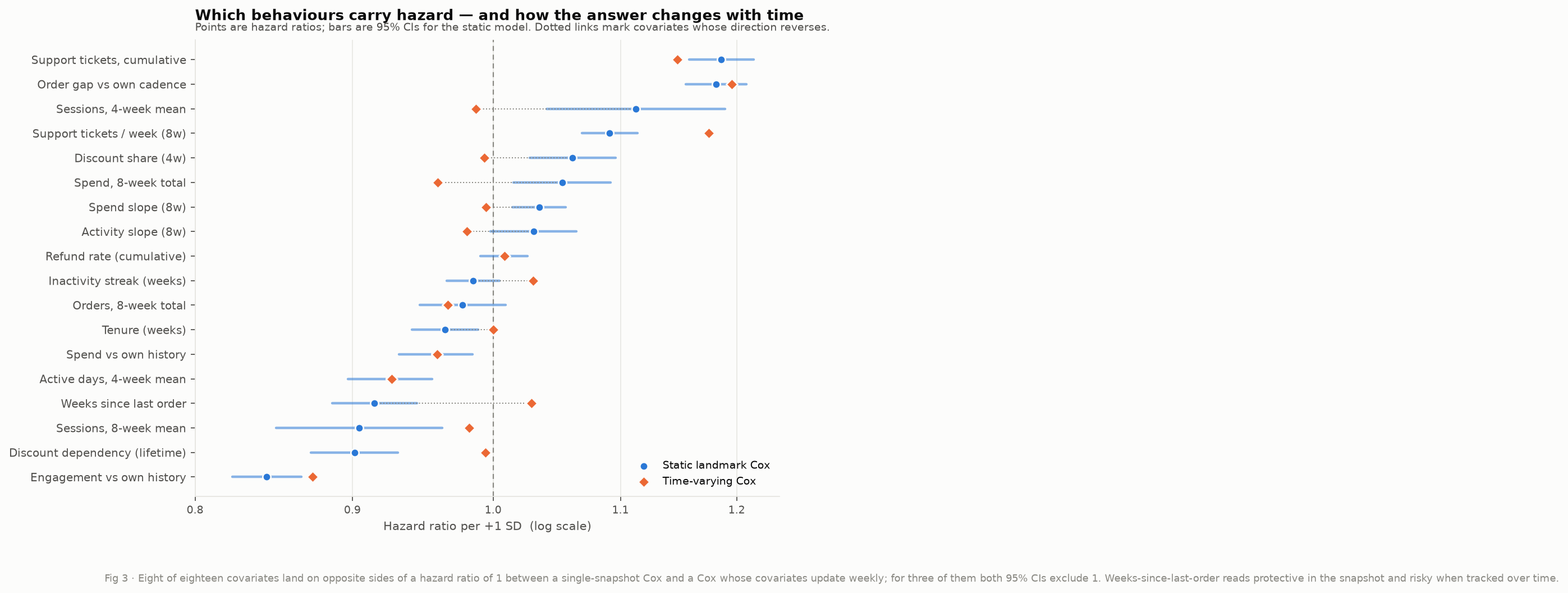
Some covariates point the other way once you track them
Between-customer differences and within-customer change can run in opposite directions. A snapshot estimates a blend of the two.
Weeks since last order is the clearest case. In a snapshot it is dominated by who the customer is — infrequent buyers have large values and are not high risk. Tracked within a customer it measures what changed, and a gap opening relative to that person’s own cadence is associated with higher hazard.
Reported as a longitudinal-modelling result. The variance decomposition that would license the term “Simpson’s paradox” was not performed.
| Covariate | Snapshot HR | Time-varying HR | Both CIs exclude 1 |
|---|---|---|---|
| Sessions, 4-week mean | 1.113 | 0.987 | supported |
| Weeks since last order | 0.915 | 1.029 | supported |
| Spend, 8-week total | 1.053 | 0.959 | supported |
| Discount share (4w) | 1.061 | 0.994 | no |
| Activity slope (8w) | 1.031 | 0.980 | no |
| Inactivity streak (weeks) | 0.985 | 1.030 | no |
| Spend slope (8w) | 1.035 | 0.995 | no |
| Tenure (weeks) | 0.965 | 1.000 | no |
Highlighted rows are the 3 reversals where each direction is individually distinguishable from no effect. The remaining rows include covariates that are simply null in one of the two models — those have not reversed, and quoting the loose count alone would overstate the result.
Why the panel is simulated
The real candidate was downloaded and profiled before the decision, not assumed away.
UCI Online Retail II is a genuine two-year weekly panel — 1,067,371 invoice lines, 5,942 identified customers. Profiled directly, it supplies 3 of 7 required behavioural signals. It has no sessions, support_tickets, discount_share — and no an observed churn event.
The deeper problem is the endpoint. In a non-contractual retailer there is no churn event, only an absence of orders, so any label must be imposed by an inactivity rule. That makes the target partly deterministic in a predictor such as recency — a circular evaluation in which every reported C-index measures the labelling rule rather than behaviour. With a median inter-purchase gap of 24.95 days, no threshold separates “churned” from “slow”.
And on real data the mechanisms are unobserved, so the blind-recovery test below — the load-bearing evaluation here — would be unfalsifiable.
Calibrated, not invented
The simulation is calibrated to selected empirical quantities from UCI Online Retail II, while retaining synthetic mechanisms needed for controlled survival and trajectory experiments. It is not a realistic reproduction of that population in every respect.
| Quantity | Simulated | Real |
|---|---|---|
| Refund value share of gross | 0.0561 | 0.0617 |
| Median inter-order gap (days) | 14 | 24.95 |
The order gap deliberately departs: at a wholesale retailer’s cadence a weekly panel is ~90% empty. Even so, 82.0% of simulated customer-weeks contain no order.
4 trajectory types, partially recovered
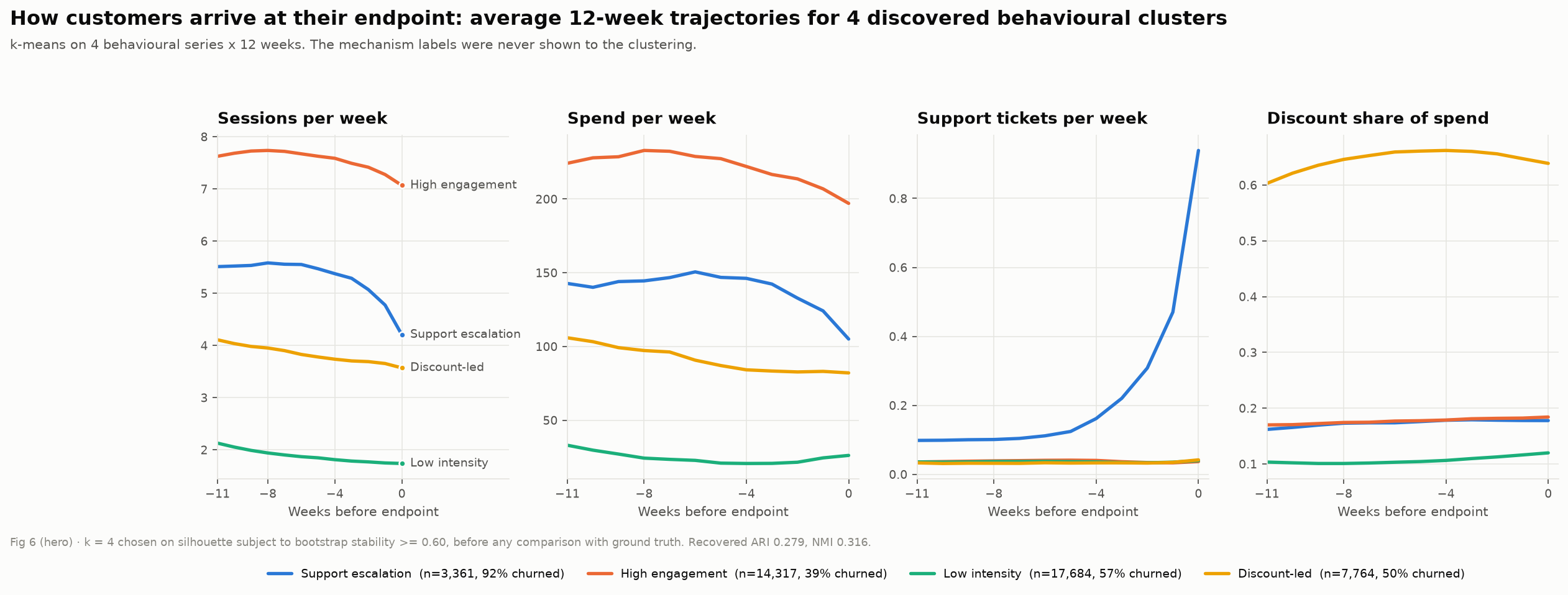
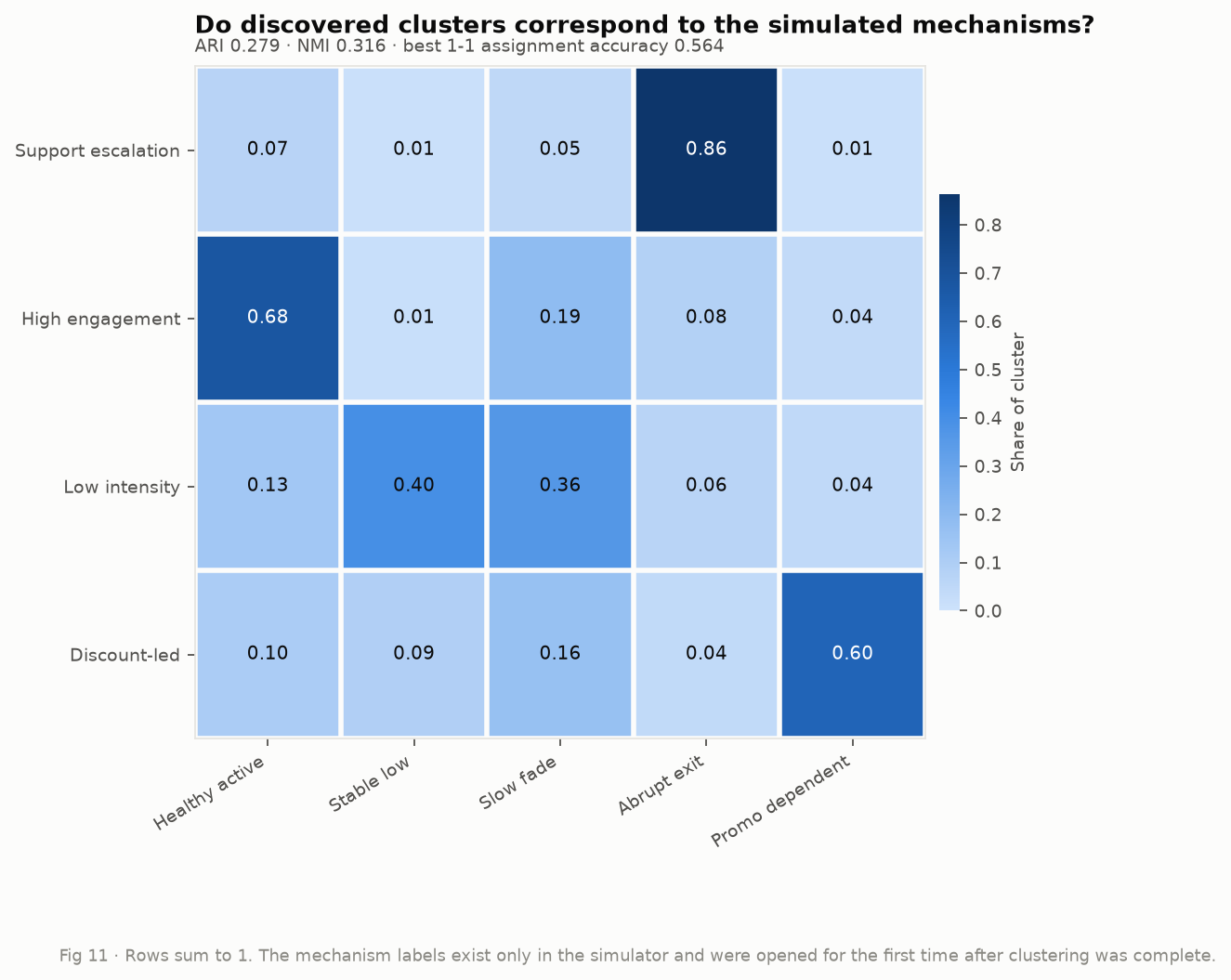
k was chosen on silhouette subject to a bootstrap-stability floor, before the mechanism labels were opened. A test asserts statically that the choice precedes the truth file being read.
| Cluster | n | Churned | Dominant mechanism | Purity | Recall | Median warning |
|---|---|---|---|---|---|---|
| Support escalation | 3,361 | 92% | abrupt exit | 0.864 | 0.524 | 1 wk |
| High engagement | 14,317 | 39% | healthy active | 0.677 | 0.738 | 10 wk |
| Low intensity | 17,684 | 57% | stable low | 0.397 | 0.882 | 15 wk |
| Discount-led | 7,764 | 50% | promo dependent | 0.603 | 0.785 | 14 wk |
Purity and recall are not the same number
“Support escalation” is 86.4% abrupt exits — almost everything in it is one mechanism — but it contains only 52.4% of all abrupt exits. It is a precise description of a route and a partial census of the customers taking it. Reporting either figure alone would misrepresent the result.
The informative failure
“Low intensity” is only 60.3% pure: it mixes stable-low and slow-fade customers, and absorbs 78.5% of the former. A slow decline viewed through its terminal 12-week window has already declined, so it resembles a customer who was always quiet. The information that separates them lies before the window. The clusters were not relabelled to hide this.
The warning horizon is not a constant
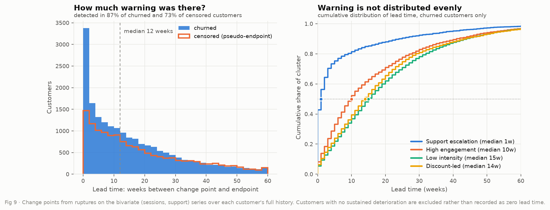
Change points from ruptures over each customer’s full history, validated against the simulation’s hidden onsets — one of the concrete advantages of a controlled design.
A sustained deterioration is detected in 86.8% of churned customers and 73.0% of censored ones. That gap is the detector’s specificity, and it is modest.
The observable warning horizon differs by a factor of fifteen across routes. For the highest-risk cluster the median is one week, and more than half get one week or less — a weekly scoring cadence would reach most of them after the fact, no matter how accurate the score.
No claim is made that an intervention within that horizon would succeed. The point is that the horizon itself is not a constant, and a single average lead time describes none of these groups.
A good ranking that cannot say how risk arose
A conventional binary classifier, built the usual way including the usual mistake: 2,842 customers (10.1%) have follow-up ending before the horizon and are labelled “did not churn”.
Who is in the top risk decile (n = 848)
| True mechanism | Share |
|---|---|
| slow fade | 39.4% |
| abrupt exit | 26.3% |
| healthy active | 16.5% |
| stable low | 9.8% |
| promo dependent | 8.0% |
These customers share a score. They do not share a mechanism, and from the section above they do not share a response window: the slow fades have a median of 14 weeks of visible warning, the abrupt exits 1.
A static score can rank customers reasonably well while remaining operationally ambiguous about how risk emerged and how much warning time exists.
Model class was the smaller lever
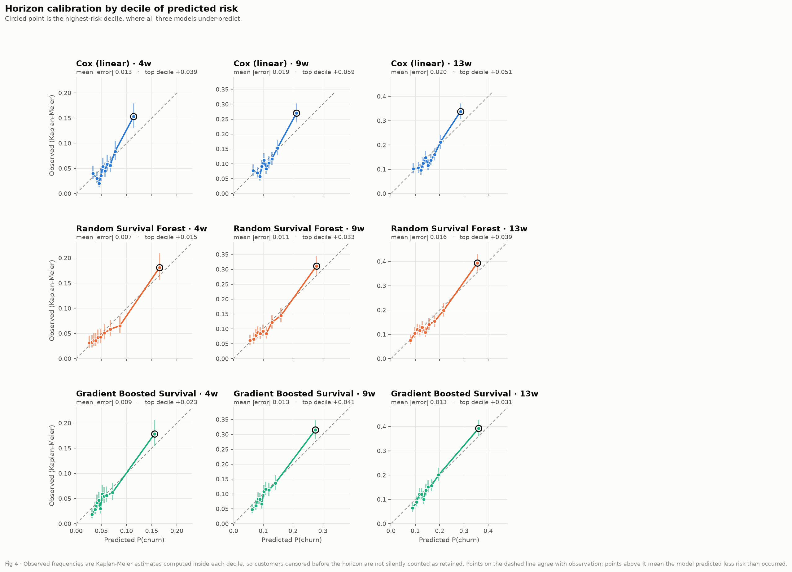
Same cohort, same design matrix, same split, no per-model tuning.
| Model | Harrell’s C | Integrated Brier | Fit time | Top-decile miss |
|---|---|---|---|---|
| Cox (linear) | 0.594 | 0.1748 | 1.4s | +0.059 |
| Random Survival Forest | 0.618 | 0.1702 | 3 min | +0.039 |
| Gradient Boosted Survival | 0.622 | 0.1694 | 22 min | +0.041 |
The spread across model classes (0.028 in C-index) is smaller than the gain from changing the time representation (0.072). Calibration is good in the bulk but every model under-predicts the highest-risk decile, with the prediction falling outside the within-decile Kaplan-Meier confidence interval in all nine model-horizon cells. Monotone rank ordering is not calibration.
Proportional hazards is violated for 11 of 18 covariates (scaled Schoenfeld residuals, rank time-transform, α = 0.05, no multiplicity correction). Stratifying the baseline hazard on the worst violator reduces that to 6 of 17 at a concordance cost of 0.596 → 0.591.
What failed first
Three initial choices were wrong. They are preserved as scored comparisons rather than quietly corrected, because the correction is the evidence that the method was tested.
Absolute inactivity streak
Did: Hazard driven by raw consecutive zero-order weeks made customers who buy rarely always look overdue.
Cost: Inverted the stable-low mechanism into the highest-risk group, at a 96% event rate.
Fixed by: Inactivity measured against each customer's own habitual inter-order gap.
Change-point detector
Did: Detecting on the session series alone, smoothed, with a minimum segment of 3.
Cost: Placed abrupt exits a median of 13 weeks before the endpoint when the true incident was 1 week before.
Fixed by: Bivariate raw (sessions + support tickets) with min_size = 1, scored against the hidden onsets: correlation with the true incident week rose from 0.573 to 0.760.
Eight-week value estimator
Did: Expected value from trailing 8-week spend.
Cost: Zero for 33.97% of customers, because 82% of customer-weeks contain no order — the entire bottom value tercile would have been identically zero.
Fixed by: Lifetime spend rate up to the scoring week; zero for 9.3%.
Change-point configurations, scored against the hidden onsets
| Configuration | Detected | r with true incident week | Abrupt-exit lead | True lead |
|---|---|---|---|---|
| final: bivariate, raw, min_size=1 | 86.8% | 0.760 | 2 wk | 1 wk |
| sessions only, raw, min_size=1 | 82.7% | 0.573 | 13 wk | 1 wk |
| bivariate, 4-week smoothed, min_size=1 | 79.6% | 0.633 | 6 wk | 1 wk |
| bivariate, raw, min_size=3 | 79.0% | 0.744 | 5 wk | 1 wk |
Being able to score a detector against a known onset is one of the things a controlled simulation buys. On real data none of these rows could be computed.
Ranking revenue at risk — and what that does not license
Priority = P(churn within 13 weeks) × expected 13-week value. Of the top 1,000 by risk alone and the top 1,000 by priority, only 28.9% are the same customers.
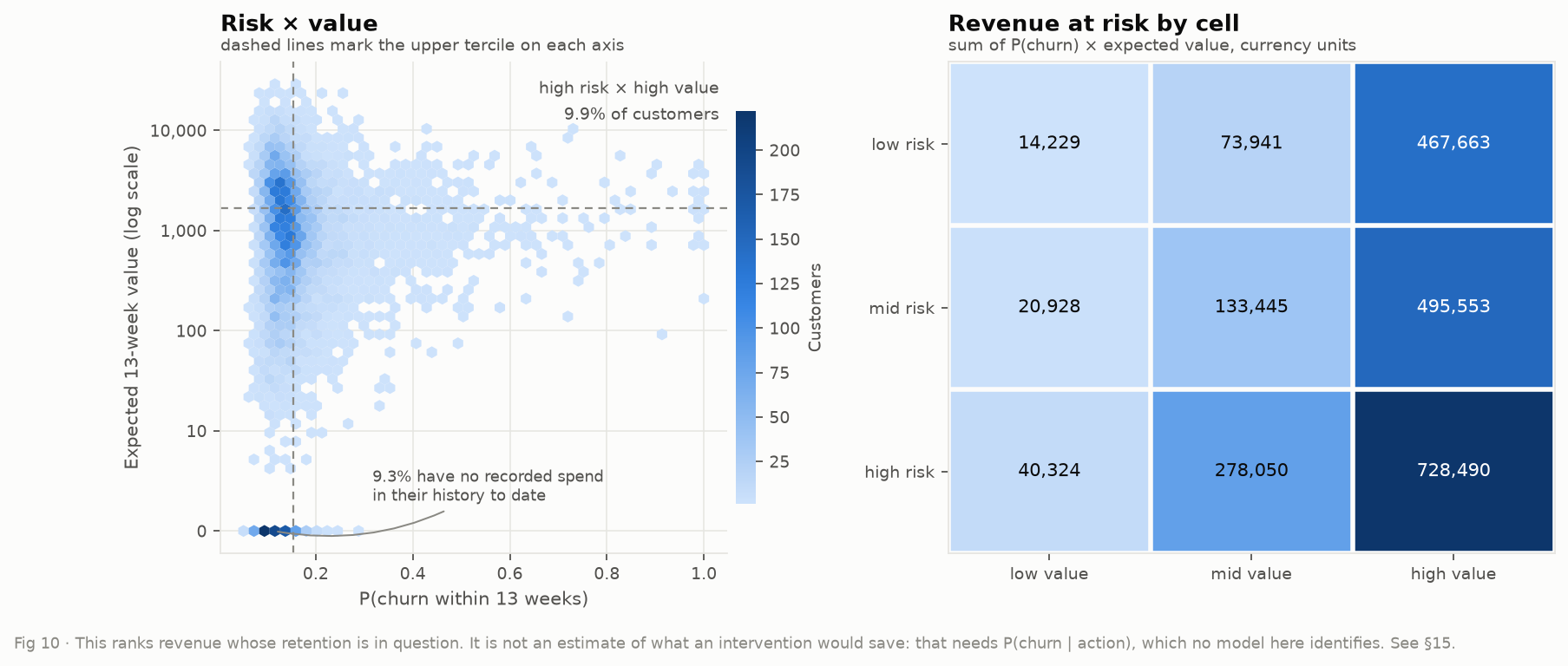
- Some of the highest-priority customers are already gone. The support-escalation cluster has the highest mean churn probability and a median warning of one week.
- Intervention can be negative for some customers. Contacting a quiet but content customer can prompt the cancellation they were not considering; a risk ranking cannot separate them from the persuadable.
- The promo-dependent cluster is a trap that will look like a success. Its members churn during promotional droughts. Send them a discount and engagement recovers — as it would have when the next promotion ran anyway.
What this study does not establish
- The primary experiment uses synthetic data. The recovery result shows the method recovers mechanisms of the kind simulated — a necessary test, not evidence about any real business.
- Calibration against real data is partial, covering order value, refund rate and loosely purchase timing. The inter-order gap deliberately differs.
- The churn mechanisms were intentionally designed. Real customers mix routes, switch routes, and respond to events no latent state here represents.
- Clustering quality depends on the feature window; the 12-week endpoint-aligned view collapses slow-fade and stable-low.
- Customers who churned inside their first twelve weeks are excluded from the trajectory analysis, so it says nothing about early-life churn.
- PH violations are substantial (11/18) and only partly remedied.
- Model performance is moderate — C-index 0.594–0.622 against an oracle ceiling of 0.676.
- Hazard relationships in simulated data are associations by construction, not automatically real-world causal relationships.
- No retention intervention is tested. Risk × value prioritisation is not uplift modelling.
- Customers churn once; real customers lapse and return. Voluntary churn, involuntary churn and dormancy are pooled rather than treated as competing risks.
Two levels of verification
Everything on this page is read from persisted stage outputs. Nothing is fitted on request.
Fast — about a minute
git clone https://github.com/Gariyuuu/customer-404
cd customer-404
make setup
make test      # 82 tests, regenerates nothing
The suite runs its own small simulation, so it verifies the generator’s invariants without the 2,431,369-row panel on disk. With artefacts present it also re-derives every headline number in the report and checks it still appears there.
Full rebuild — about 35 minutes
make all       # stage 0 through the figures
make help      # stage by stage
The gradient-boosted survival fit alone is ~22 minutes: scikit-survival evaluates the Cox partial-likelihood gradient in O(n²) per boosting stage, measured at ~5.4 s per stage on 19,804 training rows. Use the full rebuild only when persisted results are missing or verification detects an inconsistency.